8. Spatio-temporal Variograms

With version 1.1, SciKit-GStat implements the SpatioTemporalVariogram class. It replaces the SpaceTimeVariogram, which is deprecated now. The main difference is the input data: the old class needed a complete grid of time series, one for each location. The new class takes one row per observation, with the spatial coordinates followed by the time:

x, y, [z, ...], time

Thus, the observations can be located freely in space and time, which is the common case for real sensor networks with missing values or different sampling schedules. The time can be given as numbers or as datetime-like objects.

The spatio-temporal data is derived from Fersch et al. (2020). From that data publication, the wireless sensor network data is used. The originally published 15 minutes intervals soil temperature data at 20 cm depth was aggregated to mean hourly values. Here, only 10 stations and every 12th hour is used, as the number of observation pairs grows quadratically with the number of observations. The data is published under Creative Commons BY 4.0 license. Please cite the original publication if you use the data, and not SciKit-GStat.

References

Fersch, Benjamin, et al. “A dense network of cosmic-ray neutron sensors for soil moisture observation in a pre-alpine headwater catchment in Germany.” Earth System Science Data Discussions 2020 (2020): 1-35.

import skgstat as skg
import numpy as np
import pandas as pd
import json
import warnings
import matplotlib.pyplot as plt
warnings.filterwarnings('ignore')

8.1 Load data

Load the TERENO soil temperature data from Fersch et al. (2020):

with open('./tereno_fendt/tereno.json', 'r') as js:
    data_obj = json.load(js)

coords = np.array(data_obj['coordinates'])
vals = np.array(data_obj['values'])
print(data_obj['description'])

Data derived from Fersch et al. (2020) https://doi.org/10.5194/essd-2020-48. Published under CC BY 4.0.
 It is  From the WSN product, the T_a in 20cm depth is extracted

The data starts at May 1st, 2019. Use every 5th station and every 12th hour.

coords = coords[::5][:10]
vals = vals[::5][:10, ::12][:, :18]
times = pd.date_range('2019-05-01', periods=vals.shape[1], freq='12h')

8.2 From a grid

The data is a grid of time series, as used by the old SpaceTimeVariogram. The from_grid method converts each grid cell into one observation.

STV = skg.SpatioTemporalVariogram.from_grid(coords, vals, times=times, x_lags=6, t_lags=8)
print('Observations: %d' % STV.values.size)
print('Pairs: %d' % STV.bin_count.sum())

Observations: 180
Pairs: 16110

8.3 Observations

To illustrate irregular observations, we remove every 5th observation from the grid. The result is a table with one row per observation, which cannot be represented by the old grid interface anymore.

df = pd.DataFrame({
    'x': np.repeat(coords[:, 0], len(times)),
    'y': np.repeat(coords[:, 1], len(times)),
    'time': np.tile(times, len(coords)),
    'temperature': vals.flatten()
})
df = df.iloc[np.arange(len(df)) % 5 != 0].dropna()
print(df.head())

              x             y                time  temperature
1  5.078272e+06  1.560321e+06 2019-05-01 12:00:00      18.1425
2  5.078272e+06  1.560321e+06 2019-05-02 00:00:00      17.3850
3  5.078272e+06  1.560321e+06 2019-05-02 12:00:00      18.2425
4  5.078272e+06  1.560321e+06 2019-05-03 00:00:00      17.4825
6  5.078272e+06  1.560321e+06 2019-05-04 00:00:00      17.6675

The time is the last coordinate column. Datetime-like time is anchored at the oldest timestamp and converted into seconds. All lags are calculated in seconds, therefore maxlag_time is given in seconds as well. Only the plots convert the time axis into the unit of the data resolution.

STV = skg.SpatioTemporalVariogram(
    df[['x', 'y', 'time']],
    df['temperature'],
    x_lags=6,
    t_lags=8,
    maxlag_time=4 * 24 * 60 * 60
)
print('Time origin: %s' % STV.time_origin)
print('Time unit: %s' % STV.time_unit)

Time origin: 2019-05-01 00:00:00
Time unit: hours

8.4 Experimental variogram

Each space and time lag class combination has its own number of point pairs. Check the bin count before interpreting the experimental variogram.

print(STV.bin_count)

[[340 238 222 214 220 184 164 148]
 [391 252 237 215 186 185 173 158]
 [392 251 234 212 198 179 173 156]
 [239 141 132 127 122 110  97  88]
 [ 98  60  57  55  44  47  41  38]
 [132  82  78  73  62  63  56  52]]

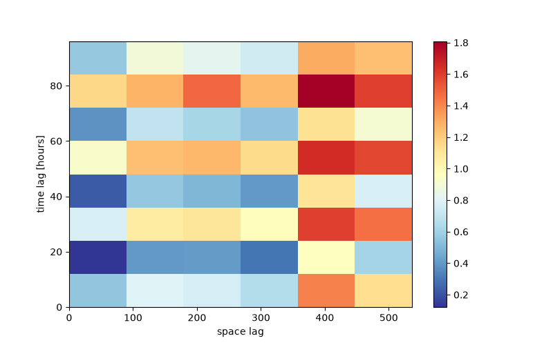
The matrix plot shows the experimental variogram for each lag class.

fig = STV.plot(kind='matrix', figsize=(8, 5))

8.5 Fitting

The product-sum model fits the marginal models for space and time first. Then, its three parameters are fitted to the experimental variogram.

STV.fit()
print(STV.cof)

[0.33804767 1.11481519 0.55956454]

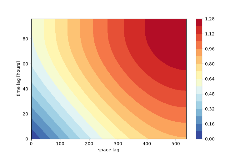
Once fitted, the contour plots show the model.

fig = STV.plot(kind='contourf', figsize=(8, 5), levels=15)

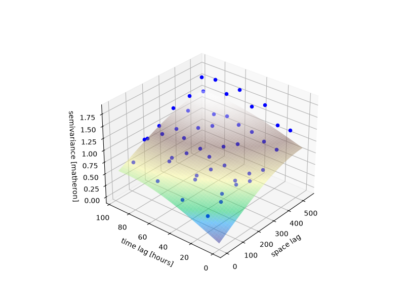
The 3D plot shows the experimental variogram along with the model.

fig = STV.plot(kind='scatter', figsize=(8, 6))